

Theory · Image and measurement · The wave
The wave: a front that propagates.
In SeedCounter, one click on a seed is enough for the outline to appear. From the click, a region grows through the seed and stops at the edge. This page tells that story the way mathematics tells it: a front that moves fast where the color is similar and slowly where it is not, the algorithm that computes the front, and what happens when two seeds touch.
Go deeper · mathematics and references
The idea
Think of a fire that starts at the clicked point and spreads across the image. Where the color of a pixel is similar to that of the click, the fire runs. Where the color changes, it almost stops. After a time \(t\), the burned area is the seed, and the line of fire is at its edge.
Growing a region from a point chosen by a person is an old idea in image processing [1]. What mathematics adds is treating the growth as a front: knowing at what instant the front reaches each pixel, solving that quickly and understanding why it stops.
Definition
Let \(T(x)\) be the instant at which the front starting from the click reaches pixel \(x\). The region reached by time \(t\) is the sublevel set \(\{x : T(x)\le t\}\), and the front at time \(t\) is its boundary, the level curve \(\{T=t\}\). Knowing \(T\) is knowing all the fronts at once.
The color cost
For the fire to know where to run, each pixel needs a number saying how far its color is from the color of the click. SeedCounter uses the color difference \(\Delta E^*_{ab}\) of the CIELAB color space, standardized in 1976 [2]: the straight-line distance between two colors in the coordinates \(L^*\) (lightness), \(a^*\) (green to red) and \(b^*\) (blue to yellow).
where \((L^*_0,a^*_0,b^*_0)\) is the mean color of the 5 × 5 pixel window around the click. The mean removes the noise of a single pixel. In the crop of Figure 1, the click lands on the light seed coat of the upper seed, with reference color \(L^*=54{,}0\), \(a^*=10{,}8\), \(b^*=6{,}1\). The median distance of the blue paper from it is \(\Delta E=51{,}1\). The red embryo of the same seed is at 32.2. There are finer formulas for color difference, such as CIEDE2000 [3], but to separate seed from paper the Euclidean distance is enough.
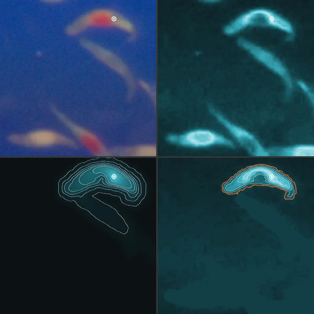 photo and clickΔE to the clickarrival time Twave level
Arrival time and the eikonal equation
Give each pixel a speed \(F(x)\gt0\), high where the color is similar to that of the click and low where it is not. Moving a stretch \(ds\) through a pixel of speed \(F\), the front takes \(ds/F\). The arrival time at \(x\) is that of the fastest path:
with \(\gamma\) traversed by arc length. From \(x\), a step \(h\) in the best direction increases \(T\) by \(h/F(x)\), and in no direction does it increase less. This says that the derivative of \(T\) in the direction of steepest growth equals \(1/F\):
This is the eikonal equation, the same as in geometric optics, where \(F\) plays the role of the inverse of the refractive index. In general it has no differentiable solution: where two optimal paths tie, \(T\) has a kink. The right notion of solution is that of viscosity solutions, due to Crandall and Lions, and for positive \(F\) the viscosity solution of (3) is exactly the shortest time (2) [4].
In Figure 1 the speed is \(F=1/\big(1+(\Delta E/\kappa)^4\big)\), with \(\kappa=18\): it drops to half when the color moves 18 units away from the click. On the paper, the median of \(F\) is 0.015, about 66 times slower than at the color of the click. The level curves crowd together at the edge because the front slows down there. But they do not stop: the reached area goes from 4,636 pixels at \(T=200\) to 6,169 at 400, 8,314 at 800 and 15,553 at 1,600. With the sum, the front never stops on its own. Someone has to choose when to stop, and the choice of \(\kappa\) changes the answer.
Fast marching and Dijkstra
To compute \(T\) on a pixel grid, Sethian's fast marching method copies the idea of Dijkstra's algorithm for shortest paths in graphs [5][8]. The pixels fall into three groups: accepted, with a final \(T\); the band, neighbors of the accepted ones with a provisional \(T\); and the far ones. At each step, the band pixel with the smallest \(T\) is accepted, and its neighbors recompute their own values. With a priority queue, the total cost is \(O(N\log N)\) for \(N\) pixels.
The difference is in the neighbor's calculation. In Dijkstra, the neighbor receives \(T(u)+w(u,v)\): the front only moves along the edges of the grid. In fast marching, the neighbor solves a discrete version of (3), with the smallest accepted values \(a\) horizontally and \(b\) vertically:
and \(T=\min(a,b)+1/F\) otherwise. The square root lets the front move diagonally without following the edges. Tsitsiklis reached the same kind of algorithm by another route, that of optimal trajectories in control [7]. Fronts as level sets of a function come from the work of Osher and Sethian [6].
true circleDijkstra, 4 neighborsDijkstra, 8 neighborsfast marching
Simulation
Figure 2. With speed 1 everywhere, the level curve \(T=70\) from a point should be a circle of radius 70 pixels. Dijkstra with 4 neighbors draws a diamond and with 8, an octagon. Fast marching comes out almost round.
Result · Dijkstra's grid error
With 8 neighbors and steps of length 1 and \(\sqrt2\), the distance measured to a point at angle \(\theta\in[0,45°]\) is \(r\,(\cos\theta+(\sqrt2-1)\sin\theta)\). The maximum of this ratio is \(\sqrt{1+(\sqrt2-1)^2}=\sqrt{4-2\sqrt2}\approx1{,}0824\), at \(\tan\theta=\sqrt2-1\), that is, \(\theta=22{,}5°\). With 4 neighbors the ratio is \(\cos\theta+\sin\theta\), with maximum \(\sqrt2\) at 45°. The error does not depend on the pixel size, so refining the grid does not remove it.
| method | radius 20 px | radius 45 px | radius 95 px | radius 190 px |
|---|---|---|---|---|
| Dijkstra, 8 neighbors | 8,24% | 8,24% | 8,24% | 8,24% |
| fast marching | 4,51% | 2,59% | 1,48% | 0,87% |
The table shows the largest relative error on a ring of each radius, measured on the grids of this page. Dijkstra's stays flat at 8.24%, the value from the calculation above, and fast marching's falls when the same distance spans more pixels. With 4 neighbors, the maximum error is 41.42%.
The SeedCounter wave: the worst stretch
The SeedCounter wave does not add up the cost along the path. It looks at the worst stretch: the cost of a path is the largest \(\Delta E\) it passes through, and the value of a pixel is that of the best path to it.
The computation is the usual Dijkstra with the maximum in place of the sum: the neighbor \(v\) of an accepted pixel \(u\) receives \(\max\big(T_\infty(u),\Delta E(v)\big)\). The name \(T_\infty\) recalls an intuition: if the cost of a stretch were \(\Delta E^p\) and that of a path the \(p\)-th root of the sum, for large \(p\) only the largest term would count.
Result · the region is a connected component
For every level \(t\), the region \(\{x: T_\infty(x)\le t\}\) is the connected component of the set \(\{x:\Delta E(x)\le t\}\) that contains the click.
Proof. If \(x\) is in that component, there is a path from the click to \(x\) inside \(\{\Delta E\le t\}\), and its worst stretch is at most \(t\): hence \(T_\infty(x)\le t\). If \(T_\infty(x)\le t\), the optimal path never exceeds \(t\), so it lies entirely inside \(\{\Delta E\le t\}\) and connects \(x\) to the click. \(\square\)
The front of the wave is then a level curve of \(\Delta E\) itself, with no distance propagated through the grid. That is why it does not inherit the diamond or the octagon of Figure 2. On a synthetic field in which \(\Delta E\) grows with the distance to the center, so that the target is a perfect disk, the region of the wave came out round: the radii at 0° and 45° differ by less than 0.5%. The wave uses 4 neighbors on purpose. With 8, two seeds that touch only at the corner of a pixel would be stitched into one.
Where the wave stops: the escape level
As \(t\) is raised gradually, the region grows through the seed until, at a certain level, it escapes into the paper and takes over the image. That level is the escape cost:
This is the formula of the mountain pass theorem of Ambrosetti and Rabinowitz, \(c=\inf_{\gamma}\max_t J(\gamma(t))\), with the landscape \(J=\Delta E\) [9]. Picture the click at the bottom of a valley: among all the paths that leave the valley, the best one is the one that climbs least, and its highest point is the pass, a saddle of the landscape. Their theorem guarantees, in function spaces and under compactness conditions, that this level is a critical value. Here only the formula is borrowed, in the image plane.
In the crop of Figure 1, \(c^*=48{,}2\). Up to \(\Delta E\le48{,}20\) the region has 5,699 pixels, the whole seed with the embryo. At \(\Delta E\le48{,}22\) it has 30,670 pixels: it went through the pass and into the paper. The wave stops just below that level. With the worst stretch, the stopping criterion comes from the image itself, and no \(\kappa\) needs to be chosen.
On the real plate
The instrument below starts at the click of Figure 1, with the maps computed in Python, and redoes everything in your browser. Click another seed to change the starting point. In sum mode, the control is the time \(t\) and \(\kappa\) changes the speed. In worst-stretch mode, the control is the level \(\Delta E\), and the orange line on the chart marks the escape level.
Instrument · the front over the real plate
Times and levels are computed on the 320 × 320 px crop, with a 4-pixel neighborhood in both modes. In sum mode, the front slows down at the edge and keeps going. In worst-stretch mode, the area jumps at the escape level.
Touching seeds and the mountain pass
When two seeds touch, the mask becomes a single blob and the question becomes where to cut. Here another front comes in: the one that starts at the edge of the blob and moves inward, with speed 1. Its arrival time is the distance map \(d(x)\), the distance from each pixel to the background, the solution of \(|\nabla d|=1\) with \(d=0\) on the border. It is equation (3) with \(F\equiv1\).
Each seed becomes a hill on the distance map, with its peak near the middle. Two touching seeds give two peaks, and between them a saddle, at the waist where they touch. The mountain pass theorem says that every path from one peak to the other descends at least to the level
which is the same formula (6), with \(J=-d\). The point where the best path reaches this level is the saddle, and the cut line passes through it. The watershed finds this line by flooding \(-d\) from the peaks: the two basins meet at the saddle [10].
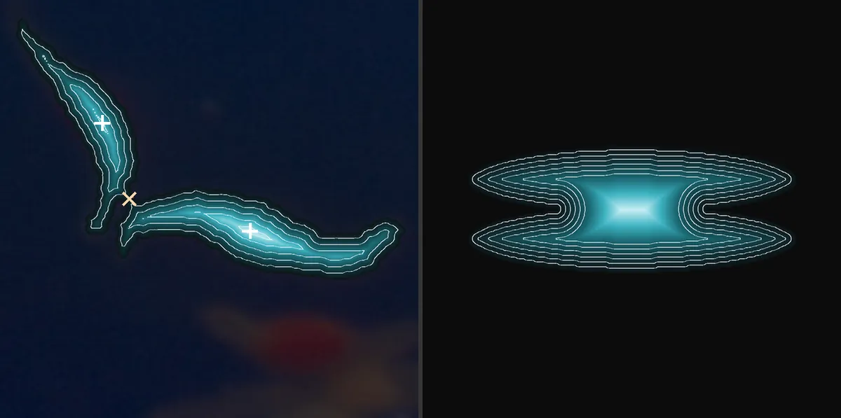 two real seedssynthetic pair, side by side
In the seed on the right there is a third peak, of 15.0 px, separated from the main one by a saddle of 14.0 px: a waist of only 6.7%. An elongated seed has a ridge in the distance map, and the ridge has bumps. To avoid cutting one seed in half, only the peaks whose saddle lies well below them count. In mathematical morphology this is the h-maxima transform, computed by reconstruction [11].
Where the saddle vanishes
The right side of Figure 3 shows the case that breaks the recipe. Two elongated seeds lying side by side do not form a waist between their centers. The union is fatter in the middle, the distance there is greater than at the center of each seed, and the map has a single ridge. There is no saddle, and the distance map has no cut to propose.
Figure 4 measures when this happens. For two equal ellipses of the same area, side by side with their major axes parallel, the depth of the waist is \(1-d_{\text{sela}}/d_{\text{pico}}\), computed from the geometry of the ellipses, without any pixels. The overlap is the fraction of the width by which one seed extends over the other.
With 11% overlap, the waist is 54.4% for round seeds (L/W 1.0), 36.0% for L/W 1.5, 17.1% for 2.2 and 1.4% for 3.5. At L/W 3.96 it vanishes. The limit is not a constant: it depends on elongation and overlap together, a boundary in two variables. An orchid seed, with an L/W ratio near 3.5, falls squarely in the region where the distance map stops helping.
When the saddle vanishes, the information for the cut does not disappear: it moves to the outline. At the ends of the pair two indentations appear, visible in the right-hand panel of Figure 3, and the natural cut joins one to the other. Methods that look for these concave points were compared by Zafari and colleagues [12]. The boundary in Figure 4 gives a rule that can be computed before trying: with the L/W ratio of the seeds in the scene, one can tell whether the distance map still has a saddle to offer. This rule is a proposal and has not been implemented yet.
In SeedCounter
In SeedCounter
When you click on a seed, the app takes the mean color of the 5 × 5 pixel window around the click, computes the \(\Delta E^*_{ab}\) from each pixel to that color, and grows the region by the worst stretch, with a 4-pixel neighborhood, within a window around the click. The wave stops a little below the escape level of that window, and the outline appears as a proposal. The person checks, accepts or corrects. When the selected outline covers two touching seeds, the app proposes splitting them, and the person chooses between Split and Keep. The cut line is not editable yet: if it runs in the wrong place, the way out is to draw the outline by hand. Fast marching is not in the app: the wave does not need it, because it does not propagate distance. A sum-based front could help follow a weak edge without leaking, but this is a proposal and has not been tested.
Where it fails
A seed with little contrast against the background has a low escape level: the wave stops early or escapes into the paper. Two touching seeds of the same color end up in the same region, because the path between them does not cross a different color, and the cut has to come from other information. For elongated seeds side by side, the distance map has no saddle, as in Figure 4. And the edge of an out-of-focus seed is a color ramp: the level at which the wave stops decides where on the ramp the outline falls.
Data
Dataset "Sementes de Orquídeas" v8, Roboflow Universe (universe.roboflow.com/sementes-de-orqudea/sementes-de-orquideas), license CC BY 4.0. Crops of orchid tetrazolium plates, scale in pixels only. The figures, the instrument maps and the numbers come from site/_src/figuras/teoria-imagem-onda.py. Figure 4 is a simulation with ellipses.
References
- Adams R., Bischof L. (1994). Seeded region growing. IEEE Transactions on Pattern Analysis and Machine Intelligence 16(6), 641–647. doi:10.1109/34.295913
- Robertson A. R. (1977). The CIE 1976 color-difference formulae. Color Research & Application 2(1), 7–11. doi:10.1002/j.1520-6378.1977.tb00104.x
- Sharma G., Wu W., Dalal E. N. (2005). The CIEDE2000 color-difference formula: implementation notes, supplementary test data, and mathematical observations. Color Research & Application 30(1), 21–30. doi:10.1002/col.20070
- Crandall M. G., Lions P.-L. (1983). Viscosity solutions of Hamilton-Jacobi equations. Transactions of the American Mathematical Society 277(1), 1–42. doi:10.1090/S0002-9947-1983-0690039-8
- Sethian J. A. (1996). A fast marching level set method for monotonically advancing fronts. Proceedings of the National Academy of Sciences 93(4), 1591–1595. doi:10.1073/pnas.93.4.1591
- Osher S., Sethian J. A. (1988). Fronts propagating with curvature-dependent speed: algorithms based on Hamilton-Jacobi formulations. Journal of Computational Physics 79(1), 12–49. doi:10.1016/0021-9991(88)90002-2
- Tsitsiklis J. N. (1995). Efficient algorithms for globally optimal trajectories. IEEE Transactions on Automatic Control 40(9), 1528–1538. doi:10.1109/9.412624
- Dijkstra E. W. (1959). A note on two problems in connexion with graphs. Numerische Mathematik 1, 269–271. doi:10.1007/BF01386390
- Ambrosetti A., Rabinowitz P. H. (1973). Dual variational methods in critical point theory and applications. Journal of Functional Analysis 14(4), 349–381. doi:10.1016/0022-1236(73)90051-7
- Vincent L., Soille P. (1991). Watersheds in digital spaces: an efficient algorithm based on immersion simulations. IEEE Transactions on Pattern Analysis and Machine Intelligence 13(6), 583–598. doi:10.1109/34.87344
- Vincent L. (1993). Morphological grayscale reconstruction in image analysis: applications and efficient algorithms. IEEE Transactions on Image Processing 2(2), 176–201. doi:10.1109/83.217222
- Zafari S., Eerola T., Sampo J., Kälviäinen H., Haario H. (2017). Comparison of concave point detection methods for overlapping convex objects segmentation. In Image Analysis (Lecture Notes in Computer Science), 245–256. Springer. doi:10.1007/978-3-319-59129-2_21
One click, one front, one outline.
In SeedCounter, the wave proposes the outline of each seed and you check it.