

Theory · Image and measurement · The threshold
The threshold: Otsu and the histogram.
Before counting, the machine decides, pixel by pixel, what is seed and what is paper. The simplest way is a single number: above it, seed. This page shows how Otsu's method picks that number from the histogram alone, why the color channel changes the result, and in which images the calculation misleads.
Go deeper · mathematics and references
The idea
In a photo of a tetrazolium plate there are two kinds of pixel: seed and blue paper. If each pixel becomes a number, the histogram of those numbers usually has two humps, one for the paper and one for the seeds. Choosing the threshold means choosing where to cut the valley between them.
In 1979, Nobuyuki Otsu proposed a criterion with no parameters at all [1]. For each possible cut, the histogram is split into two classes. The best cut is the one that makes the two classes differ most in their means, weighted by how many pixels each has. The animation Live segmentation runs this calculation on one seed.
Definition
Let \(I:\Omega\to\mathbb{R}\) be an image channel, one number per pixel. A global threshold is a single number \(t\), the same for the whole image, that defines the mask \(M_t=\{x\in\Omega : I(x)\gt t\}\). The pixels in \(M_t\) are called seed and the others, background.
Before the histogram, a channel
The photo has three numbers per pixel (red, green and blue) and the threshold needs one. The choice of that number decides much of the result. Three candidates make sense for a light seed on blue paper.
Gray is the video luma, \(Y'=0{,}299R+0{,}587G+0{,}114B\): the seed is lighter than the paper. The \((R+G)/2-B\) channel measures how much more red and green than blue a pixel has: high on the cream seed coat and the red embryo, strongly negative on the paper. The third is b*, the yellow-to-blue axis of the CIELAB color space, standardized in 1976 [5]:
where \(Y\) and \(Z\) come from the linear R, G and B values through a fixed matrix, and \(Y_n\), \(Z_n\) are those of the reference white. Blue paper has a strongly negative b*. Cream or red seed sits well above it.
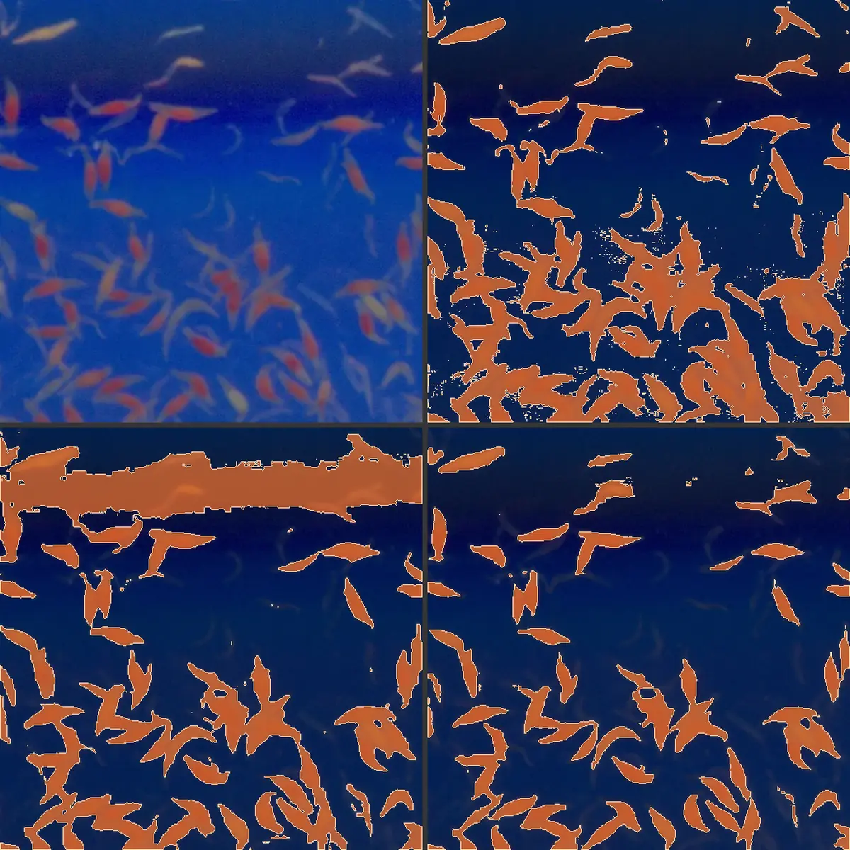 photoOtsu on grayOtsu on (R+G)/2 − BOtsu on b*
What defeats gray is uneven light. In this crop, the paper in the shadow strip has a gray value of 43.0 and the paper below has 59.6. The typical seed has 87.6. The light moves the paper by 16.6 levels out of a margin of 28 to the seed, more than half of it, and the Otsu threshold (66) ends up a few levels from the light paper. On b*, the same shadow moves the paper from −50.6 to −38.5, or 12.1 units, out of a margin of 36.7 to the seed (−13.9): one third.
The reason lies in formula (1) itself. If the light on the paper is multiplied by \(k\), the linear values X, Y and Z are too, and \(b^*\) ends up multiplied by \(k^{1/3}\). The paper stays on the blue side, closer to zero but still far from the seed. Shadow mainly changes lightness, and b* measures color.
This does not make b* a champion. In the Where it fails section, the \((R+G)/2-B\) channel holds up better on an image with few seeds, because on this plate the paper is smoother in it. The right channel is the one that separates the seed from the paper in units of the paper's noise and changes little when the light changes.
Otsu's calculation
Once the channel is chosen, each pixel falls into one of \(L\) histogram bins (here \(L=256\)). Let \(p_i\) be the fraction of pixels in bin \(i\). A cut at \(k\) separates the bins \(0,\dots,k\) (background) from the bins \(k+1,\dots,L-1\) (seed).
Definition
Weights \(\omega_0(k)=\sum_{i\le k}p_i\) and \(\omega_1=1-\omega_0\). Means \(\mu_0=\frac{1}{\omega_0}\sum_{i\le k}i\,p_i\) and \(\mu_1=\frac{1}{\omega_1}\sum_{i\gt k}i\,p_i\), with overall mean \(\mu_T=\omega_0\mu_0+\omega_1\mu_1\). Variances \(\sigma_0^2\) and \(\sigma_1^2\) of each class, within-class variance \(\sigma_W^2=\omega_0\sigma_0^2+\omega_1\sigma_1^2\), total variance \(\sigma_T^2=\sum_i (i-\mu_T)^2p_i\) and between-class variance
Result 1 · variance decomposition
For every cut \(k\), \(\;\sigma_T^2=\sigma_W^2(k)+\sigma_B^2(k)\). Since \(\sigma_T^2\) does not depend on \(k\), maximizing \(\sigma_B^2\) is the same as minimizing \(\sigma_W^2\).
Proof. For \(i\) in class \(c\), write \(i-\mu_T=(i-\mu_c)+(\mu_c-\mu_T)\). Squaring and summing with weights \(p_i\) within the class, the cross term is \(2(\mu_c-\mu_T)\sum_{i\in c}p_i(i-\mu_c)=0\), by the definition of \(\mu_c\). What remains is \(\sigma_T^2=\sum_c\omega_c\sigma_c^2+\sum_c\omega_c(\mu_c-\mu_T)^2=\sigma_W^2+\sigma_B^2\). The second form of (2) comes from \(\mu_0-\mu_T=\omega_1(\mu_0-\mu_1)\) and \(\mu_1-\mu_T=\omega_0(\mu_1-\mu_0)\): the sum equals \(\omega_0\omega_1(\omega_1+\omega_0)(\mu_0-\mu_1)^2\). \(\square\)
The Otsu threshold is \(k^*=\arg\max_k\sigma_B^2(k)\). The two pieces of the histogram end up as tight as possible around their means, and the means as far apart as possible. Otsu himself proposed measuring how good the separation is by \(\eta=\sigma_B^2(k^*)/\sigma_T^2\), a number between 0 and 1 that does not change if the channel is multiplied by a constant or shifted by another [1].
Two values give \(\eta\) its scale. A single Gaussian, cut at the mean, gives \(\eta=2/\pi\approx 0{,}637\): that is what the method finds when there are no two classes. Two narrow, distant classes take \(\eta\) close to 1. In the crops on this page, with seeds, \(\eta\) falls between 0.65 and 0.78.
A single pass
Recomputing means and variances for each of the 256 cuts would be wasteful. With the cumulative sums \(\omega(k)=\sum_{i\le k}p_i\) and \(\mu(k)=\sum_{i\le k}i\,p_i\), formula (2) becomes
because \(\mu_0=\mu/\omega\), \(\mu_1=(\mu_T-\mu)/(1-\omega)\) and \(\mu_0-\mu_1=(\mu-\omega\mu_T)/\big(\omega(1-\omega)\big)\). Each cut costs a single calculation. The whole method is one pass over the pixels to build the histogram and one pass over the bins. This is what runs in the instruments below:
// h: histogram with 256 bins; returns the cut k*
let n = sum(h), mT = Σ i·h[i]/n, w = 0, m = 0, best = -1, kStar = 0;
for (let i = 0; i < 256; i++) {
  w += h[i]/n;  m += i*h[i]/n;              // accumulated ω(k) and μ(k)
  const sB = (mT*w - m)**2 / (w*(1 - w));   // equation (3)
  if (sB > best) { best = sB; kStar = i; }
}
The threshold sits midway between the means
Result 2 · fixed point
For a continuous histogram with density \(p\), at an interior maximum of \(\sigma_B^2\) the threshold satisfies \(\;t^*=\tfrac12\big(\mu_0(t^*)+\mu_1(t^*)\big)\).
Sketch. Write \(\sigma_B^2=N^2/D\) with \(N=\mu_T\omega_0-\mu(t)\) and \(D=\omega_0(1-\omega_0)\). Since \(\omega_0'=p(t)\) and \(\mu'(t)=t\,p(t)\), we have \(N'=p(t)(\mu_T-t)\) and \(D'=p(t)(1-2\omega_0)\). Setting the derivative of \(N^2/D\), with \(N\ne0\), to zero gives \(2(\mu_T-t)\,\omega_0\omega_1=N(\omega_1-\omega_0)\). Substituting \(N=\omega_0\omega_1(\mu_1-\mu_0)\) and \(\mu_T=\omega_0\mu_0+\omega_1\mu_1\) leaves \(2t=(\omega_0+\omega_1)(\mu_0+\mu_1)=\mu_0+\mu_1\). \(\square\)
On the instrument's clean plate, in b*, the two classes of the Otsu cut have means −41.52 and −12.42. The midpoint is −26.97, and the Otsu threshold is −27.0.
This is the same fixed point as the iterative method of Ridler and Calvard [4]: start from any threshold, compute the two means, put the threshold midway between them and repeat. Among the fixed points, Otsu takes the one with the largest \(\sigma_B^2\). The result also explains the failures. The threshold only sees the means. The width of each class and its size matter only through how they shift the means.
On the real plate
The instrument below loads five real crops, computes the three channels in your browser and shows the mask, the histogram and the \(\sigma_B^2(t)\) curve. The Otsu button jumps to the maximum of the curve. The Minimum error button uses the criterion from the Alternatives section.
Instrument · the threshold on the real plate
backgroundseedσ2B(t), on its own scalethreshold
The histogram is on a square-root scale so that the seed hump shows up next to the paper hump. Everything runs in your browser, on the same images as the figures.
On the full plate, the three channels agree: Otsu marks 26.8% of the image on b*, 28.8% on \((R+G)/2-B\) and 28.8% on gray. On the shadow strip, \(\eta\) is practically the same in all three channels (0.654, 0.659 and 0.654) and the masks are very different, as in Figure 1. \(\eta\) measures the histogram, and the histogram does not know where each pixel is.
On the plate glare, all three channels get it wrong (30.0% to 37.1% of the image), because the glare strip is lighter than the paper and, in part, more yellow. On the paper-only crop, Otsu still returns a threshold and marks between 41.5% and 49.6% of the image as seed, with \(\eta\) between 0.60 and 0.66, close to the \(2/\pi\) of a single Gaussian. The method always answers, and the answer does not say whether there was anything to find.
Where it fails
Few seeds on a large background
To isolate the effect of class size, Figure 2 builds histograms from real pixels of one plate: 8,817 pixels from inside the annotated seeds and 223,729 pixels from a quadrant with no seed. The mixture is exact, the weighted sum of the two histograms, for each seed fraction. Only the proportion changes.
The jump has a calculation behind it. Take a small seed fraction \(f\), the difference \(\Delta\) between the seed and paper means, and the standard deviation \(\sigma\) of the paper. The right cut gives \(\sigma_B^2\approx f\,\Delta^2\) by equation (2). Cutting the paper in half, if it is close to Gaussian, gives \(\sigma_B^2\approx\frac{2}{\pi}\sigma^2\). Otsu switches cuts when the second passes the first:
| channel | Δ | paper σ | Δ/σ | predicted breakdown point | measured breakdown point |
|---|---|---|---|---|---|
| gray | 51,5 | 4,31 | 11,9 | 0,45% | 0,51% |
| b* | 48,0 | 1,67 | 28,6 | 0,078% | 0,086% |
| (R+G)/2 − B | 107,1 | 2,88 | 37,1 | 0,046% | 0,042% |
The estimate ignores the width of the seed class and gets the breakdown point right within 13%. What matters is the ratio \(\Delta/\sigma\), the distance between seed and paper in units of the paper's noise. On this plate each seed takes up about 0.4% of the 946 × 946 px crop: on gray, a crop with a single seed is already below the breakdown point.
Instrument · few seeds
Lower the fraction slowly and watch the σ2B(t) curve: it has two bumps, one in the valley between paper and seed and the other in the middle of the paper hump. When the second passes the first, Otsu jumps.
Uneven light and glare
A global threshold assumes the paper has the same value across the whole image. The shadow and glare in Figure 1 and in the instrument break that assumption, and no method that looks only at the histogram fixes it, because the histogram has lost the position of the pixels.
A histogram without two humps
With a single class, as in the paper crop, Otsu cuts the noise in half. With weak contrast, the two humps merge and the valley disappears. In both cases the method returns a number with the same confidence as always.
Where it fails
The Otsu threshold assumes a histogram with two humps, classes of comparable size and uniform paper. On this plate, with real pixels, it breaks down below 0.51% seed on gray, 0.086% on b* and 0.042% on (R+G)/2 − B. With shadow or glare, it fails on any channel that confuses the uneven paper with seed. On a crop with no seed, it marks close to half of the image.
Alternatives
Minimum error
Kittler and Illingworth modeled each class as a Gaussian with its own mean, variance and weight and chose the cut that best explains the histogram under that model [2]. The criterion is
and the threshold is the \(k\) that minimizes \(J\). Because the width of each class enters the calculation, the small class does not lose to the large one. On the mixture in Figure 2, minimum error does not jump: on b*, with 1% seed, it marks 1.02%. On the real crops, though, it fails in another way. On the shadow strip, on gray, it marks 0.4% of the image and misses almost all the seeds. On the paper crop, on b*, it marks 89%. When the histogram does not have the shape of two Gaussians, the model has nothing to hold on to.
Gaussian mixture
The smooth version of the same model fits the two Gaussians with the EM algorithm and cuts where the two weighted densities cross. The same problem shows up with another histogram in SeedCounter: that of a shape descriptor among the seeds in a scene, where isolated seeds and clusters form two humps. A two-component mixture would find that cut without a hand-picked constant. This is a proposal from the project, not yet tested.
Local threshold
Instead of one \(t\) for the image, one \(t(x)\) for each neighborhood. Sauvola and Pietikäinen use the mean \(m(x)\) and the standard deviation \(s(x)\) in a window: \(t(x)=m(x)\,[1+\kappa\,(s(x)/R-1)]\) [6]. Another way out is to flatten the light first: fit a smooth surface to the paper and subtract it, and only then apply a global threshold. Sezgin and Sankur cataloged and compared 40 thresholding methods, grouped by the information they use: histogram shape, clustering, entropy, object attributes, spatial correlation and local surface [3].
In SeedCounter
In SeedCounter
The click outline in SeedCounter is a local threshold. The person clicks on a seed, the app measures the color distance from each pixel to the color of the click and cuts that distance at a value chosen for that seed: just below the level at which the region would escape from it. Each seed gets its own threshold, which is exactly what the global histogram cannot give. The calculation is in The wave. When the person triggers "flatten background", the app fits a second-degree polynomial to the background in CIELAB by least squares, with 0-or-1 reweighting starting from the edge, so that the seeds do not pull the fit. Without this command the image stays as it was opened. The machine proposes the outline and the person checks, and it is the checking that catches the glossy paper and the pale seed.
Data
Dataset "Sementes de Orquídeas" v8, Roboflow Universe (universe.roboflow.com/sementes-de-orqudea/sementes-de-orquideas), license CC BY 4.0. Crops of orchid tetrazolium plates, scale in pixels only. The figures and numbers come from site/_src/figuras/teoria-imagem-limiar.py.
References
- Otsu N. (1979). A threshold selection method from gray-level histograms. IEEE Transactions on Systems, Man, and Cybernetics 9(1), 62–66. doi:10.1109/TSMC.1979.4310076
- Kittler J., Illingworth J. (1986). Minimum error thresholding. Pattern Recognition 19(1), 41–47. doi:10.1016/0031-3203(86)90030-0
- Sezgin M., Sankur B. (2004). Survey over image thresholding techniques and quantitative performance evaluation. Journal of Electronic Imaging 13(1), 146–165. doi:10.1117/1.1631315
- Ridler T. W., Calvard S. (1978). Picture thresholding using an iterative selection method. IEEE Transactions on Systems, Man, and Cybernetics 8(8), 630–632. doi:10.1109/TSMC.1978.4310039
- Robertson A. R. (1977). The CIE 1976 color-difference formulae. Color Research & Application 2(1), 7–11. doi:10.1002/j.1520-6378.1977.tb00104.x
- Sauvola J., Pietikäinen M. (2000). Adaptive document image binarization. Pattern Recognition 33(2), 225–236. doi:10.1016/S0031-3203(99)00055-2
A threshold for each seed, on click.
In SeedCounter, the outline comes from the color of the seed you clicked, and you check each one.