

The mean seed shape and the modes of variation.
Each outline becomes a list of 128 numbers, and 130 seeds become a matrix. The singular value decomposition of this matrix gives the mean seed shape, the directions in which shapes vary most, and how much weight each direction carries. In the seeds on this page, three directions hold 92.8% of the variation.
Go deeper · mathematics and references
The outline becomes a vector
To do algebra with shapes, each seed has to become a list of numbers of the same length. The most direct way is to walk along the outline and mark \(k\) points equally spaced in arc length, as on the Fourier page. Here \(k = 64\), and the seed becomes
Adding and subtracting these vectors only makes sense if point \(j\) of one seed corresponds to point \(j\) of another. In a seed there are almost no visible anatomical landmarks on the outline, and the equally spaced points play their role: they are Bookstein's semilandmarks [1], points defined by their position along the curve rather than by an anatomical structure. For them to correspond, one still has to choose where the outline starts, and that choice enters the alignment.
Definition
Two configurations of \(k\) points have the same shape when one becomes the other by translation, rotation and change of scale. Shape is what remains after removing these three things [2]. On this page we also remove the starting point of the outline and the mirror image, the latter because a seed can land on the plate with either face up.
Aligning before comparing
Translation is removed by subtracting the centroid. Scale is removed by dividing by the centroid size, the square root of the sum of squared distances of the points to the center, which then equals 1. Removing the rotation is the orthogonal Procrustes problem: write each seed as a matrix \(k \times 2\), with one row per point, and find the rotation \(R\) that brings \(X\) as close as possible to a reference \(M\).
Result 1 · the optimal rotation comes from a 2 × 2 SVD
If \(X\) and \(M\) are centered and \(X^\top M = U\Sigma V^\top\), the rotation that minimizes \(\lVert XR - M \rVert_F\) is
Sketch. \(\lVert XR - M\rVert_F^2 = \lVert X\rVert_F^2 + \lVert M\rVert_F^2 - 2\operatorname{tr}(R^\top X^\top M)\), and only the trace depends on \(R\). With \(Q = V^\top R^\top U\), which is orthogonal, \(\operatorname{tr}(R^\top U\Sigma V^\top) = \operatorname{tr}(\Sigma Q) = \sigma_1 q_{11} + \sigma_2 q_{22}\), and each \(\lvert q_{ii}\rvert \le 1\). The maximum is attained at \(Q = I\), that is, \(R = UV^\top\) [3]. If \(UV^\top\) is a reflection (determinant \(-1\)) and reflections are not allowed, the sign of the last column is flipped, as in (2), and the trace drops from \(\sigma_1 + \sigma_2\) to \(\sigma_1 - \sigma_2\).
With several seeds there is no given reference. Generalized Procrustes alignment [4] alternates two steps: it aligns each seed to the current mean and recomputes the mean, until the mean stops changing. Here, for each seed and in each round, we test the 64 possible starting points and the mirror image, and keep the combination with the smallest distance. With the 130 seeds, the mean stopped changing in the seventh round.
The table shows why alignment is the modeling, not a detail. These are the same 130 silhouettes, the same 64 points and the same SVD. Only the correspondence changes.
| correspondence | total variance | PC1 | PC2 | modes for 95% |
|---|---|---|---|---|
| random start, centering and scaling only | 1,004 (×31,5) | 54,3% | 42,2% | 2 |
| start at the rightmost point, no rotation | 0,040 (×1,26) | 70,5% | 17,9% | 6 |
| Procrustes alignment with starting point and mirror image | 0,032 | 88,5% | 2,6% | 5 |
With a random start, the total variance is 31.5 times larger, and the first two modes, which account for 96.5% of it, describe only where each outline starts. It looks like an excellent result (two modes are enough), but it is the worst: PCA faithfully summarizes a variation that is not shape. Figure 1 shows the two means.
The mean seed shape is the mean of the aligned vectors, \(\bar{\mathbf{x}} = \tfrac{1}{n}\sum_i \mathbf{x}_i\). After Procrustes alignment, it minimizes the sum of squared distances to the aligned seeds [2]. It differs from the average seed on the Learn page, which is the pixel-by-pixel mean of the silhouettes: the mean of outlines is an outline, and the mean of silhouettes is a heat map.
The centered matrix, the SVD and PCA
Stack the aligned seeds, each minus the mean, as rows of a matrix \(X\) of size \(n \times 2k\). Here \(n = 130\) and \(2k = 128\). Every real matrix has a singular value decomposition [6]:
with \(U\) and \(V\) having orthonormal columns and \(r\) the rank of \(X\). The columns \(\mathbf{v}_i\) live in shape space, \(\mathbb{R}^{128}\): they are directions of deformation of the outline. The columns \(\mathbf{u}_i\) live in seed space, \(\mathbb{R}^{130}\).
Result 2 · PCA is the SVD of the centered matrix
The covariance matrix of the shapes is \(S = X^\top X/(n-1)\). Then
The principal components are the columns of \(V\), the variances along them are \(\lambda_i\), and the scores of each seed on the components are the rows of \(T\) [5].
Sketch. \(X^\top X = V\Sigma U^\top U \Sigma V^\top = V\Sigma^2 V^\top\), because \(U^\top U = I\). This is already the diagonalization of \(X^\top X\) by an orthogonal matrix, and \(XV = U\Sigma V^\top V = U\Sigma\).
For the 130 seeds, \(X\) has rank 125, not 128. Three singular values are zero to machine precision (\(10^{-15}\) and below), and the corresponding directions are exactly the translations in \(x\) and in \(y\) and the rotation: the alignment has already removed those three. At most 125 modes remain.
The best rank-r approximation
Keeping only the first \(r\) terms of (3) gives \(X_r = \sum_{i \le r} \sigma_i \mathbf{u}_i \mathbf{v}_i^\top\). In terms of shapes, this approximates each seed by the mean plus a combination of the first \(r\) modes. The theorem says that no better way exists.
Eckart–Young theorem
For \(r \lt \operatorname{posto}(X)\),
Eckart and Young proved the Frobenius norm version in 1936 [7]. Mirsky extended the result to every norm invariant under orthogonal transformations, including the spectral norm [8].
Proof idea. Weyl's inequality for singular values says \(\sigma_{i+j-1}(A + C) \le \sigma_i(A) + \sigma_j(C)\) [6]. Write \(X = (X - B) + B\) with \(\operatorname{posto}(B) \le r\), so that \(\sigma_{r+1}(B) = 0\). With \(j = r + 1\) we get \(\sigma_{i+r}(X) \le \sigma_i(X - B)\) for every \(i\). Summing the squares, \(\lVert X - B\rVert_F^2 = \sum_i \sigma_i(X - B)^2 \ge \sum_i \sigma_{i+r}(X)^2 = \lVert X - X_r\rVert_F^2\). With \(i = 1\) we get the spectral version.
This is the same statement as for the truncated Fourier series: there the orthogonal basis is fixed (sines and cosines), while here the SVD chooses the orthogonal basis that best fits these seeds. Figure 2 applies the idea to a single seed.
With the mean alone, Amorpha is 6.3% away from its own outline. The first mode gets the elongation right (4.8%), and the straight side of the kidney shape appears in the second (2.4%). It lies at 4.2 standard deviations on PC2, among the farthest of the 130, which is why three modes still leave 2.4% of error. For the median of the 130 seeds, the mean alone gives an error of 6.4% and the mean with three modes, 1.4%.
Explained variance
The fraction of the variance in the first \(r\) modes is how much the Eckart and Young low-rank approximation preserves:
The first mode carries 88.5% of the variance. The first three carry 92.8%; five reach 95.0%, ten reach 97.9%, and 16 are needed for 99%. The relative error falls more slowly, because it is the square root of what is missing: with three modes, 26.8%; with ten, 14.5%.
Eigenvalues estimated from a sample carry error. By the rule of North and colleagues [9], the sampling error of \(\lambda_i\) is of the order of \(\lambda_i\sqrt{2/n}\), 12% with \(n = 130\). When two neighboring eigenvalues are closer than that, the two modes can swap places or mix from one sample to another, and only the plane they span is reliable. Here \(\lambda_2/\lambda_3 = 1{,}48\) and \(\lambda_3/\lambda_4 = 1{,}46\): the first three modes are separated. In contrast, \(\lambda_4/\lambda_5 = 1{,}19\) falls within the margin, and the fourth and fifth modes should not be read one by one.
Why compute it through the SVD
The textbook way to do PCA is to form the covariance \(X^\top X/(n-1)\) and find the eigenvectors. In exact arithmetic the result is the same as (4), but on a computer it is not. The condition number of a matrix, \(\kappa(A) = \sigma_{\max}/\sigma_{\min}\), measures how many digits a computation with it can lose.
Result 3 · forming \(A^\top A\) squares the condition number
Sketch. \(A^\top A = V\Sigma^2 V^\top\), so the singular values of \(A^\top A\) are \(\sigma_i^2\), and the ratio between the largest and the smallest is squared.
The practical consequence comes from perturbation theory [6][10]. Computing the eigenvalues of \(X^\top X\) in floating-point arithmetic, with precision \(\varepsilon\), gives each one an error of the order of \(\varepsilon\,\sigma_1^2\). In relative terms, \(\lambda_i\) can be off by as much as \(\varepsilon\,(\sigma_1/\sigma_i)^2\). The SVD of \(X\) gives each \(\sigma_i\) an error of the order of \(\varepsilon\,\sigma_1\), and the relative error in \(\sigma_i^2\) is of the order of \(\varepsilon\,\sigma_1/\sigma_i\). The covariance spends twice as many digits on the small modes.
For the 130 seeds, \(\sigma_1/\sigma_{125} \approx 2{,}6 \times 10^4\), so \(\kappa^2 \approx 6{,}9 \times 10^8\). In double precision (about 16 digits) the two routes give the same eigenvalues with a wide margin: the worst relative error through the covariance is \(1{,}6 \times 10^{-9}\). In single precision (about 7 digits), the difference appears:
| mode \(i\) | \(\sigma_1/\sigma_i\) | by the SVD of \(X\) | by the covariance |
|---|---|---|---|
| 1 | 1 | 1 × 10⁻⁸ | 2 × 10⁻⁹ |
| 50 | 127 | 4 × 10⁻⁸ | 3 × 10⁻⁵ |
| 100 | 726 | 2 × 10⁻⁷ | 4 × 10⁻⁴ |
| 120 | 4.365 | 6 × 10⁻⁷ | 5 × 10⁻³ |
| 125 | 26.305 | 4 × 10⁻⁶ | 7 × 10⁻² |
The last mode comes out with a 7% error through the covariance and 4 millionths through the SVD. For the three modes on this page, either route works. The margin disappears with worse matrices, and the classic case is least squares: the normal equation \(Z^\top Z\boldsymbol\beta = Z^\top \mathbf{y}\) also squares \(\kappa\) [10]. In the public table of Koklu and colleagues, with 106 shape and color descriptors measured on about 75,000 rice grains [11], the descriptor matrix has \(\kappa(Z) \approx 1{,}0 \times 10^5\) and the normal equation reaches \(\kappa(Z^\top Z) \approx 1{,}0 \times 10^{10}\): forming it uses up about 10 of the 16 digits of double precision. That is why the rule is to solve through the SVD (or QR), without forming \(Z^\top Z\).
The modes of variation
Each principal component is a direction of deformation. Moving \(b_i\) standard deviations along it, starting from the mean, gives
This is the point distribution model of the active shape models of Cootes and colleagues, who limit each \(b_i\) to \(\pm 3\) [12]. Drawn as images, the \(\mathbf{v}_i\) of faces became known as eigenfaces [13]. Here they are eigenseeds.
Read as shapes, PC1 is elongation: it goes from the round seed to the thin, long one, and its score has a correlation of 0.94 with the ratio of length to width. PC2 leaves one side straighter and the other more curved, the kidney shape. The two Amorpha fruticosa seeds are at +4.2 and +4.5 standard deviations on it. PC3 thins one of the ends, like an egg or a wedge, and the triangular seed of Amygdalus mongolica is at −4.6.
The seeds occupy only a part of each axis. On PC1, they range from −1.2 to +2.4 standard deviations. Model (8) is linear and keeps drawing outside that range: with \(b_1 = -2\) it gives a shape taller than it is wide, which none of the 130 has. The reason is that the distribution is not a Gaussian cloud around the mean but a set of groups (rice on one side, soybean on the other).
Instrument · deforming the mean seed shape
Click a seed on the plane, or an empty point to choose b₁ and b₂.
The mean, the three modes and the scores of the 130 seeds were computed once and are embedded in the page; the deformation (8) is done here, in your browser. Dashed is the mean seed shape; orange, the shape with weights \(b_1\), \(b_2\) and \(b_3\), in standard deviations; blue, the aligned outline of the seed chosen on the plane. When you choose a seed, the three controls move to its scores, and the difference between blue and orange is what the other 122 modes hold.
In SeedCounter
In SeedCounter
The app runs a 2 × 2 PCA on each seed. The covariance of the outline point coordinates gives the major axis, and length and width are measured along the two eigenvectors, with the seed rotated so that its major axis lies horizontal. For a symmetric 2 × 2 matrix the eigenvector has a closed form: the angle of the major axis is \(\tfrac12 \operatorname{atan2}(2s_{xy},\, s_{xx} - s_{yy})\), the same computation as the \(\theta_1\) in the Fourier normalization. In a nearly round seed the axis is poorly defined, but then length and width hardly depend on it.
The shape space on the Learn page uses the same decomposition on the whole silhouettes, pixel by pixel, and there the first mode holds about half of the variation. With aligned outlines, the first mode holds 88.5%. The representation also decides what PCA sees.
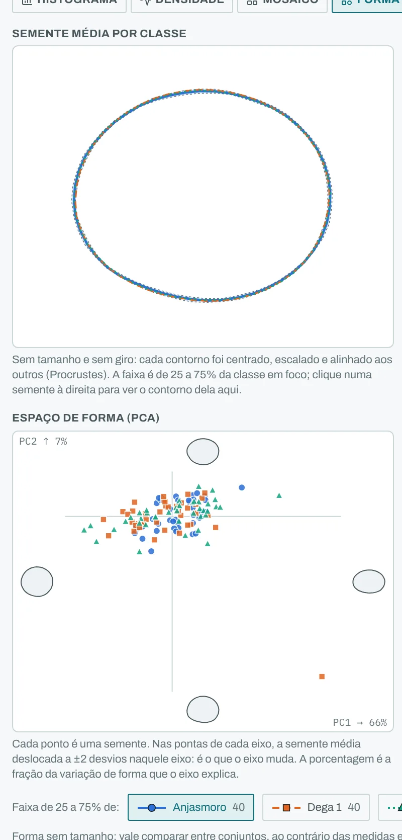
In the dataset hub, the Shape view runs this page's computation on a whole dataset: each outline resampled to 48 points, Procrustes-aligned, the mean seed shape of each class with the 25 to 75% band and the shape space of the first two modes, where clicking a point shows the seed.
Where it fails
PCA is least squares, and squaring punishes the rare. With all 145 silhouettes, including the 15 with notched outlines, PC2 rises from 2.6% to 19.3%, and five silhouettes (three native seeds with notched outlines, one broken soybean and one with a damaged seed coat) carry 81% of its variance. The second mode ends up describing five odd seeds. That is why the 15 were left out, by the criterion given below.
The model is linear and the dataset is made of groups. Large steps along a mode leave the range of the seeds, as Figure 4 shows. And the directions of greatest variance are not, in general, the ones that separate the classes: PCA shows, it does not decide. Separating classes is another problem, and the page When the line hides a class shows a case in which the simplest computation hides one of them.
Correspondence is a choice. The 64 equally spaced points do not mark the hilum or the tip of the seed. With true landmarks, the modes change.
Data
Of the 145 silhouettes of 64 × 64 px from the public SeedCounter examples (rice, soybean, coffee, corn and native species), the same ones as on the Learn page, the 130 with solidity (area over convex hull area) of at least 0.8 are included: 40 rice, 31 soybean, 28 coffee, 19 native species and 12 corn. Left out were 13 native seeds and 2 soybeans with deep notches, spines or loose pieces. The outline is the one from the Fourier page, resampled to 64 points. The script that redoes the figures is in _src/figuras/teoria-forma-svd.py.
References
- Bookstein F.L. (1997). Landmark methods for forms without landmarks: morphometrics of group differences in outline shape. Medical Image Analysis 1(3), 225–243. doi:10.1016/S1361-8415(97)85012-8
- Dryden I.L., Mardia K.V. (2016). Statistical Shape Analysis, with Applications in R, 2nd ed. Wiley.
- Schönemann P.H. (1966). A generalized solution of the orthogonal Procrustes problem. Psychometrika 31(1), 1–10. doi:10.1007/BF02289451
- Gower J.C. (1975). Generalized Procrustes analysis. Psychometrika 40(1), 33–51. doi:10.1007/BF02291478
- Jolliffe I.T., Cadima J. (2016). Principal component analysis: a review and recent developments. Philosophical Transactions of the Royal Society A 374(2065), 20150202. doi:10.1098/rsta.2015.0202
- Golub G.H., Van Loan C.F. (2013). Matrix Computations, 4th ed. Johns Hopkins University Press.
- Eckart C., Young G. (1936). The approximation of one matrix by another of lower rank. Psychometrika 1(3), 211–218. doi:10.1007/BF02288367
- Mirsky L. (1960). Symmetric gauge functions and unitarily invariant norms. The Quarterly Journal of Mathematics 11(1), 50–59. doi:10.1093/qmath/11.1.50
- North G.R., Bell T.L., Cahalan R.F., Moeng F.J. (1982). Sampling errors in the estimation of empirical orthogonal functions. Monthly Weather Review 110(7), 699–706. doi:10.1175/1520-0493(1982)110<0699:SEITEO>2.0.CO;2
- Trefethen L.N., Bau D. (1997). Numerical Linear Algebra. SIAM.
- Koklu M., Cinar I., Taspinar Y.S. (2021). Classification of rice varieties with deep learning methods. Computers and Electronics in Agriculture 187, 106285. doi:10.1016/j.compag.2021.106285
- Cootes T.F., Taylor C.J., Cooper D.H., Graham J. (1995). Active shape models: their training and application. Computer Vision and Image Understanding 61(1), 38–59. doi:10.1006/cviu.1995.1004
- Turk M., Pentland A. (1991). Eigenfaces for recognition. Journal of Cognitive Neuroscience 3(1), 71–86. doi:10.1162/jocn.1991.3.1.71
Many checked seeds become one mean shape.
SeedCounter proposes the outline of each seed and you check it. The mean and the modes come out of that set.